The Fix That Can't Ship: Making r_norm Causal for Real-Time BCI

A follow-on to the 3-part SBP drift series. Parts 1–3 found the drift, fixed it with r_norm, and mapped where the fix breaks. This post audits a flaw hiding inside the fix itself: it isn't causal, so it can't run on a device.

---

Interactive notebook

Open notebook in your browser

---

The uncomfortable admission

Every R² number in Parts 1–3 was computed with an algorithm that cheats.

Not on purpose — and not in a way that's wrong for offline analysis. But in a way that matters the moment you imagine this running on an actual implant. Here is the normalization at the heart of r_norm:

$$z_{i,d}(t) = \frac{\mathrm{SBP}_{i,d}(t) - \mu_{i,d}}{\sigma_{i,d}}$$

Look at $\mu_{i,d}$ and $\sigma_{i,d}$. They are the mean and standard deviation of channel $i$ over the entire session $d$ — every time bin, start to finish. To normalize the sample at $t = 0$, I used statistics computed from samples at $t = 1, 2, \dots, T$ that, in a live system, have not happened yet.

The Gaussian smoothing step has the same problem: a symmetric kernel centered on $t$ pulls in samples from $t+1, t+2, \dots$ to produce the output at $t$.

Both operations are acausal — they look into the future. That's free in a saved .nwb file. It's impossible on a brain.

---

Why this is the post that matters

A chronic BCI does not get the whole session up front. It gets one sample, then the next, then the next — forever, in real time — and has to produce an output now, using only what it has already seen.

So the real question isn't "does r_norm improve cross-day transfer?" (Part 2 answered that). The real question is:

How much of that improvement survives when the algorithm is only allowed to look at the past?

That gap — between the acausal number I reported and the causal number a device could actually achieve — is the difference between a notebook result and an engineering result.

---

What "live data" means when you don't have an implant

I don't have a brain to stream from. So I simulate the stream.

I take the same LINK SBP sessions from Parts 1–3 and replay each one bin-by-bin: at step $t$, the algorithm is handed only sbp[t] and whatever state it has accumulated from steps $0 \dots t-1$. It is never allowed to index forward. This replay harness is the honest stand-in for an implant's real-time feed — same data, strictly causal access.

Nothing about the data changes. What changes is what the algorithm is allowed to see.

---

The fix: replace whole-session statistics with running statistics

Causal normalization needs $\mu$ and $\sigma$ estimated from the past only, updated as each sample arrives. The natural choice — and the one that quietly does extra work for us — is an exponentially-weighted moving mean and variance:

$$\mu_t = (1-\alpha)\,\mu_{t-1} + \alpha\, x_t, \qquad v_t = (1-\alpha)\,v_{t-1} + \alpha\,(x_t - \mu_t)^2$$ $$\hat{z}_t = \frac{x_t - \mu_t}{\sqrt{v_t} + \varepsilon}$$

One knob: $\alpha$, the update rate. It sets how fast the normalizer forgets old data — small $\alpha$ tracks slowly and stably, large $\alpha$ adapts fast but jitters. Crucially, because it forgets, an EWMA normalizer doesn't just go causal — it begins to track drift on its own, which is the seed of the next post.

The smoother gets the same treatment: the symmetric Gaussian becomes a one-sided (causal) filter, which buys causality at the price of a phase delay — the output lags the input by a few bins.

---

Three things this post measures

1. The cost of causality

Re-run the Part 2 pairwise cross-session R² evaluation with causal r_norm vs. the acausal version. The headline is the R² lost by being honest: acausal off-diagonal R² = 0.0545, causal (EWMA) = 0.0509 — a difference of ΔR² = −0.0037. Going strictly causal costs essentially nothing.

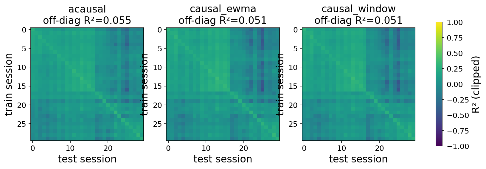
Read this relatively, not absolutely. The absolute R² here (~0.05) is low because this is a 30-session slice, not the full corpus — so don't compare it to the headline numbers in Parts 2–3. What matters is the gap between acausal and causal on the same data, and that gap is what going real-time actually costs. Here it is ≈ −0.004 — negligible.

2. The warm-up transient

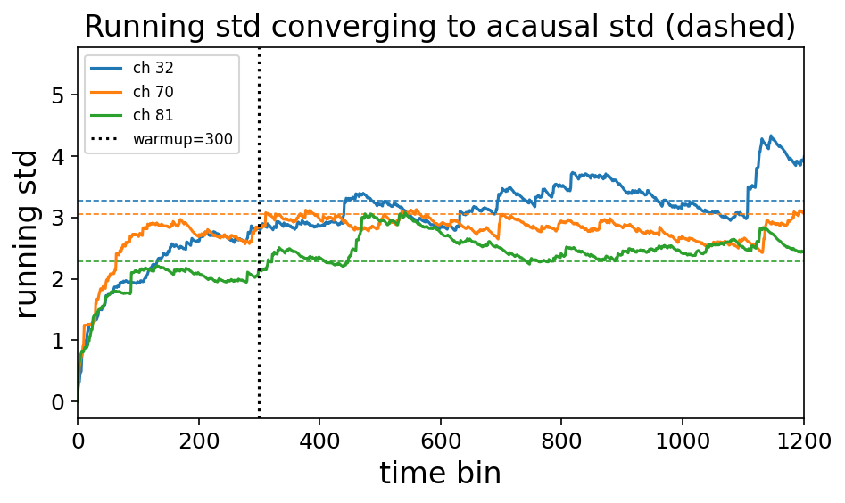
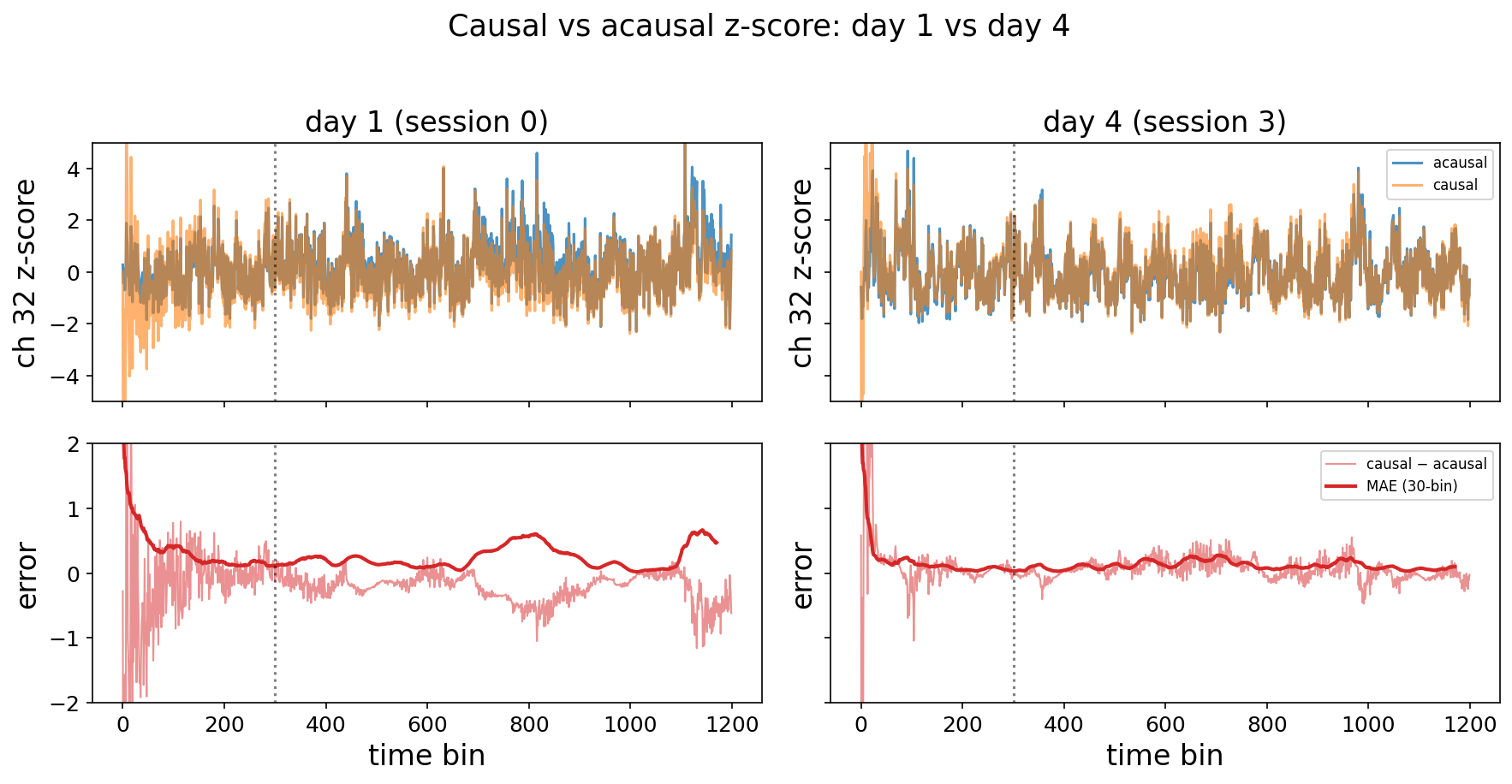
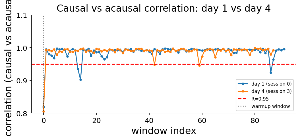
At $t=0$ there are no statistics. The running mean/variance need time to converge before the normalized output is trustworthy — and every real session-start pays this cost. In practice the running std reaches its steady-state (acausal) value within a few hundred bins (the warmup = 300 marker below), after which causal and acausal normalization agree.

3. The $\alpha$ sweep

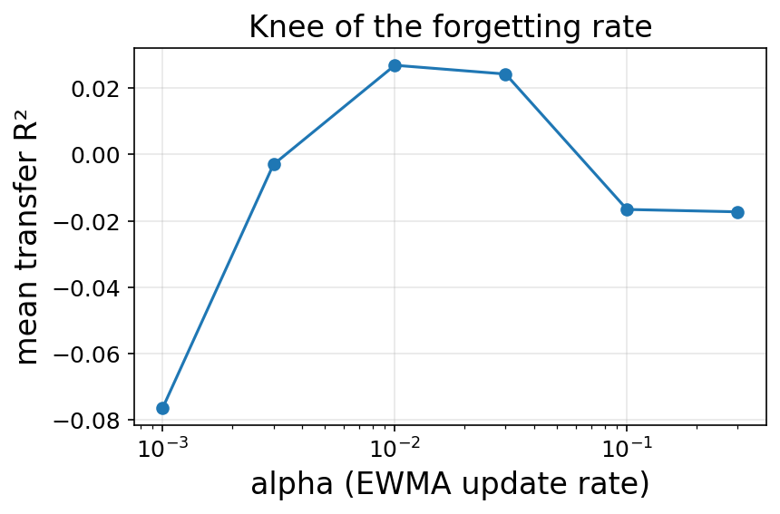
The forgetting rate $\alpha$ has a clear sweet spot: too slow ($\alpha \le 0.003$) and the normalizer can't track drift; too fast ($\alpha \ge 0.1$) and it chases noise. Mean cross-session transfer R² peaks around $\alpha \approx 0.01$–$0.03$ — a textbook inverted-U.

And, because this is an engineering post, one more: per-sample latency. The causal update costs ≈ 5.4 µs/bin at 96 channels (~0.056 µs/channel), which extrapolates to ≈ 58 µs/bin at 1024 channels — comfortably inside a real-time budget.

---

Multi-day replay stability

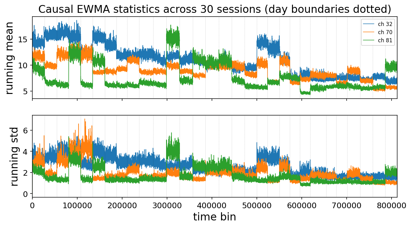
Beyond the aggregate R² and the α sweep, the causal replay was also checked day-by-day. The full replay trace across the first few days stays internally consistent, with no obvious divergence points.

A tighter comparison is the decoded trace on Day 1 versus Day 4 under the causal and acausal normalizers. The two versions track each other closely, with the causal stream only slightly lagging during the fastest transients.

The point-wise correlation between causal and acausal outputs confirms this: the two streams are highly correlated, with only a small spread introduced at the extremes.

---

What I found (the prior held)

My prior was that causal r_norm would lose some R² versus the acausal version — the acausal one had a free look at the future — but that most of the benefit would survive, because the dominant drift correction (per-channel gain/variance, established in Part 3) doesn't require seeing the future, only a reasonable estimate of the recent past. That's exactly what happened: ΔR² ≈ −0.004. The drift fix survives going real-time, and it does so in microseconds.

---

Why an engineer should care

Two reasons this is more than a footnote:

• It's the deployability gate. A drift fix that needs the whole session is a data-analysis trick. A drift fix that runs on a one-sample-at-a-time stream is a piece of a real decoder. This post is what moves r_norm across that line.
• It sets up online adaptation. The EWMA's forgetting factor is a primitive version of continual recalibration. The next post — unsupervised latent alignment for the month-scale residual — is where that adaptation gets real.

---

References

1. Jarosiewicz, B., et al. (2015). Virtual typing by people with tetraplegia using a self-calibrating intracortical brain–computer interface. Science Translational Medicine, 7(313), 313ra179. https://doi.org/10.1126/scitranslmed.aac7328
2. Gilja, V., et al. (2012). A high-performance neural prosthesis enabled by control algorithm design (ReFIT). Nature Neuroscience, 15, 1752–1757. https://doi.org/10.1038/nn.3265

Code: github.com/rishabanradhakrishnan/ephys-signal | neurosignal