Beyond the Linear Fix: A Cross-Session MLP on SBP + TCR
Part 3 of 3. Part 1 established the drift problem. Part 2 fixed the representation. This part asks whether a nonlinear joint decoder can go further.
Part 2 ended with a working result: Gold r_norm — a per-channel z-score followed by 50 ms Gaussian smoothing — shifts mean cross-day R² from −0.021 to +0.151 and eliminates the negative-transfer regime that made the static Day-0 decoder actively harmful. That's a real improvement. It's also not the ceiling.
The r_norm result used a Ridge decoder trained on a single day. A linear model trained on one session doesn't know what the signal looks like on any other day — it's just getting a better-normalized version of a distribution it still hasn't seen at training time. The logical next move is to give the decoder more sessions to learn from, and more signal to work with.
This part does both. One MLP, trained jointly on all 30 sessions, using both SBP r_norm and threshold crossing rate (TCR) z_norm as input.
The Second Feature: Threshold Crossing Rate
SBP measures power in the 300–3000 Hz band. TCR measures something different: it counts how many times each electrode's voltage dips below −4.5 × RMS in each 20 ms bin. That's a hardware-level spike detector — not spike-sorted single units, but a coarser count that fires whenever an electrode sees a large negative deflection.
The output has the same shape as SBP: (T, 96) — one value per channel per time bin, aligned on the same time axis. It's sparse: most bins are zero, and active channels fire a handful of times per second. Where SBP tracks the sustained power envelope of local neural activity, TCR is more event-like, registering individual threshold crossings.
The two features are complementary. SBP encodes mean-field activity; TCR captures phasic firing events. A decoder that sees both gets a richer description of the population state at each time point.
Normalization applied before training:
- SBP: r_norm (per-channel z-score + 50 ms Gaussian smoothing), exactly as in Part 2
- TCR: per-channel z-score within each session (z_norm)
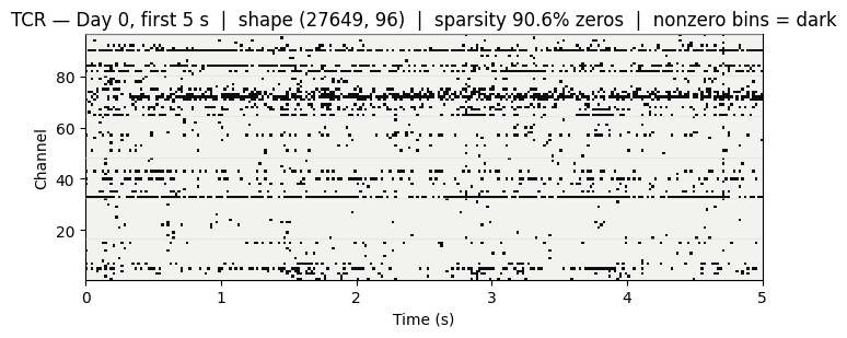
TCR is sparse — most bins are zero — while active channels show brief bursts of crossings, complementary to the smoother SBP envelope.
The Decoder
A single MLPRegressor (scikit-learn) is trained on the joint (SBP r_norm, TCR z_norm) feature matrix across all 30 sessions simultaneously. No per-session retraining. No recalibration data. The model sees every session at training time and is evaluated on all session-to-session transfer pairs.
Architecture: window=5, lag=3 (5 consecutive time bins with a 3-bin lag relative to the decoded velocity). This gives each prediction access to a 100 ms history of both feature channels, allowing the decoder to exploit temporal dynamics without explicit filter design.
The model converged in 30 iterations to a validation R² of 0.2747.
Does It Work at Short Transfer Gaps?
Before the full horizon analysis, the intuition check: decoded velocity traces at Day 5 and Day 15.
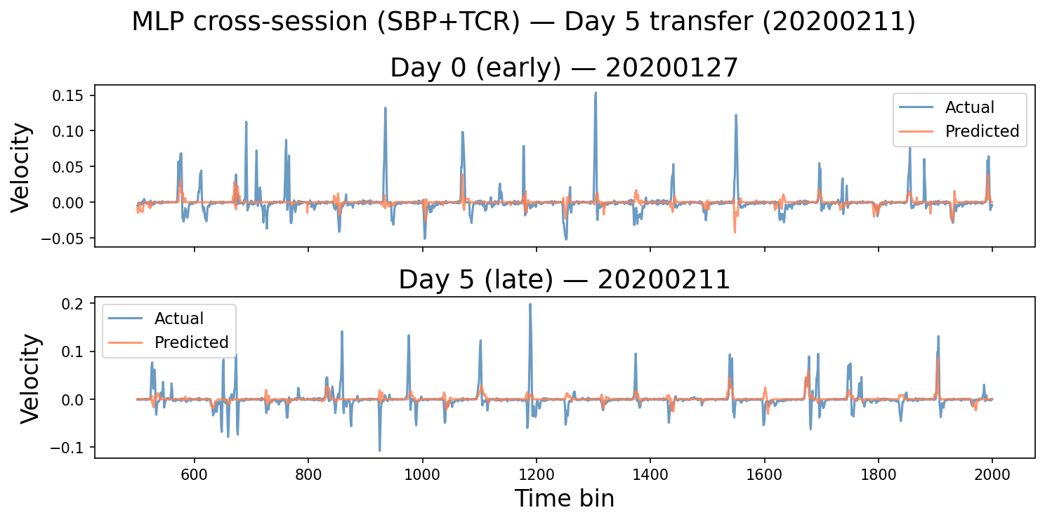
Day 5 (~2 weeks post-training-data cutoff): the MLP prediction tracks the true velocity — sign, timing, and rough amplitude are all present. This is the regime where the Ridge baseline from Part 1 was already breaking down.
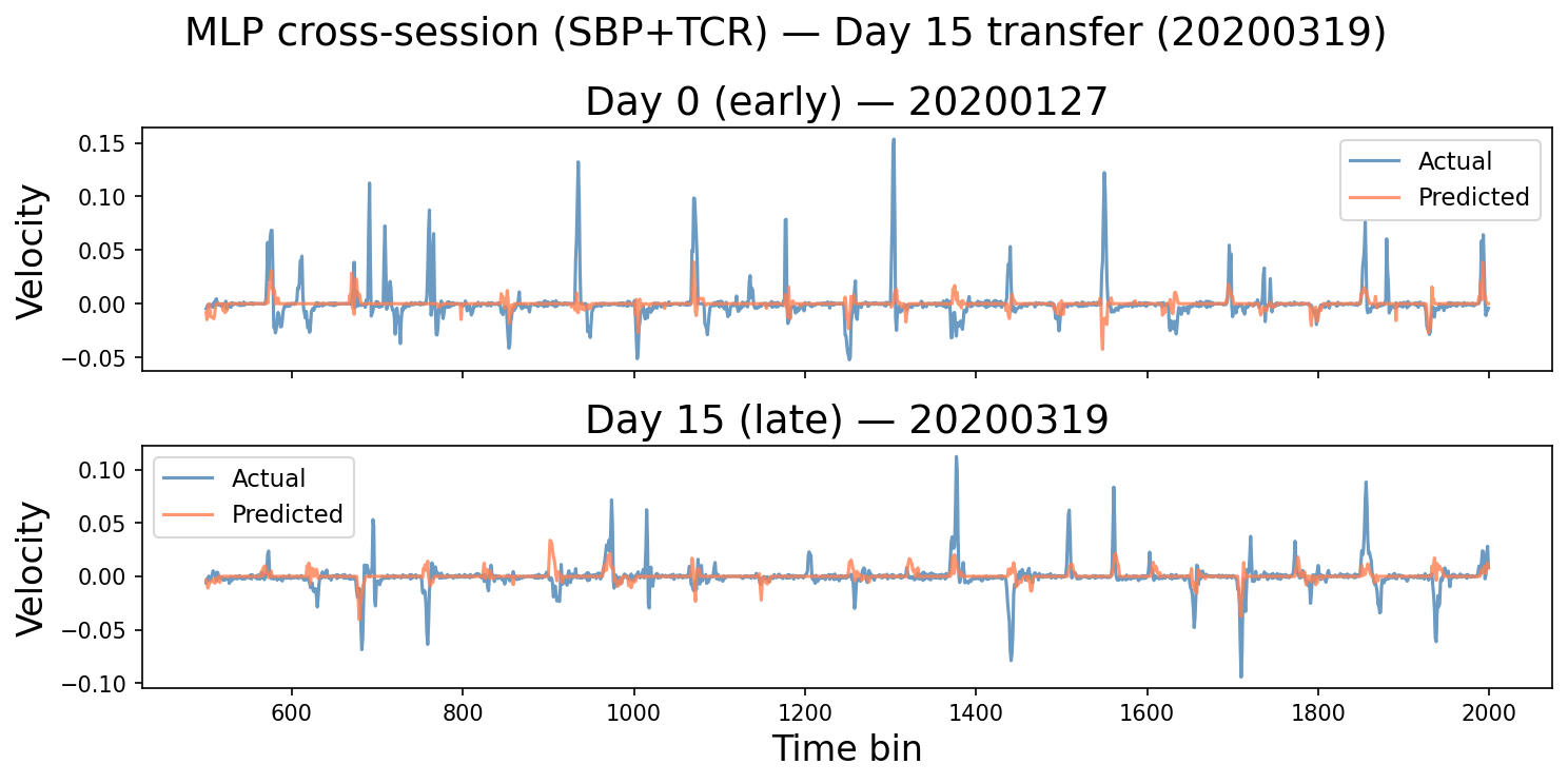
Day 15 (~one month): structure is preserved. The prediction doesn't flatten out the way the raw-SBP Ridge decoder did at comparable gaps in Part 1.
The Full Horizon Comparison
The canonical test across the series: train once, evaluate at all three time-gap bins — within a day, 1–7 days, and beyond one month.
Wide table: on a narrow screen, scroll sideways to see all columns.
| Feature set | Intra-day R² | 1–7 days | 1 month+ |
|---|---|---|---|
| r_norm Ridge (96-ch) | 0.268 | 0.104 | −0.106 |
| Raw population mean (1-ch) | 0.001 | −0.001 | −0.002 |
| MLP (SBP r_norm + TCR z_norm) | 0.387 | 0.346 | 0.360 |
The Ridge baseline from Part 2 degrades at long gaps — it still goes negative beyond one month. The MLP stays above 0.34 at every horizon, including pairs separated by more than a year.
Two figures carry the long-horizon picture. First, per-session R² across all 30 training sessions (ordered by implant day). Second, a stacked waterfall of decoded velocity for representative sessions spanning the three-year span — gray dotted true velocity, colored MLP prediction, with a 60 ms causal smoother matching real-time-style latency constraints.
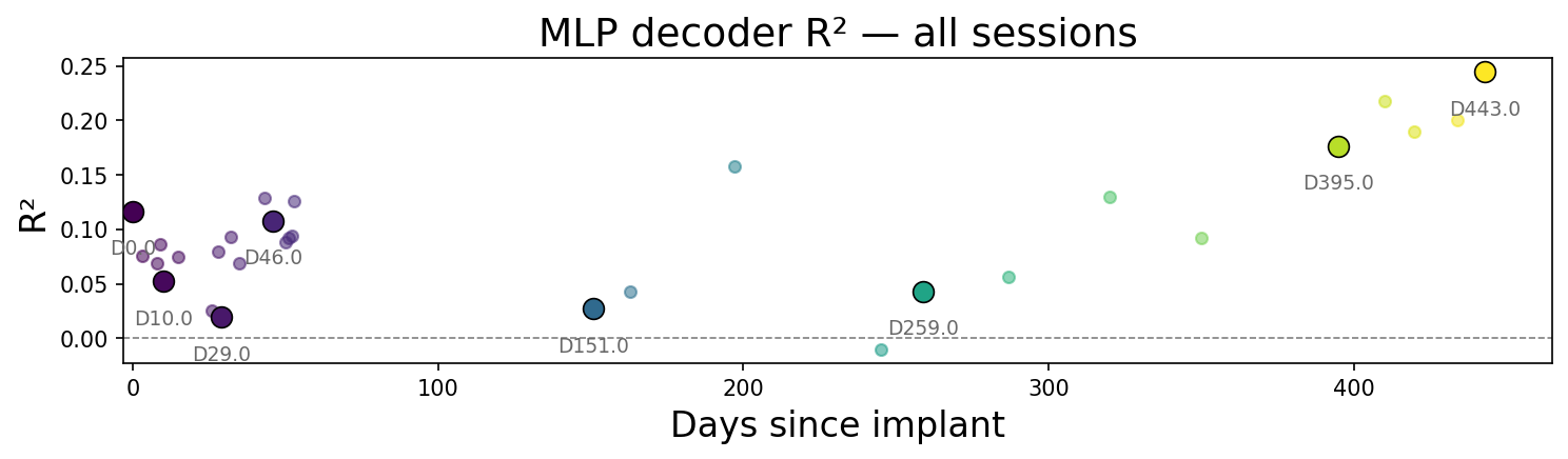
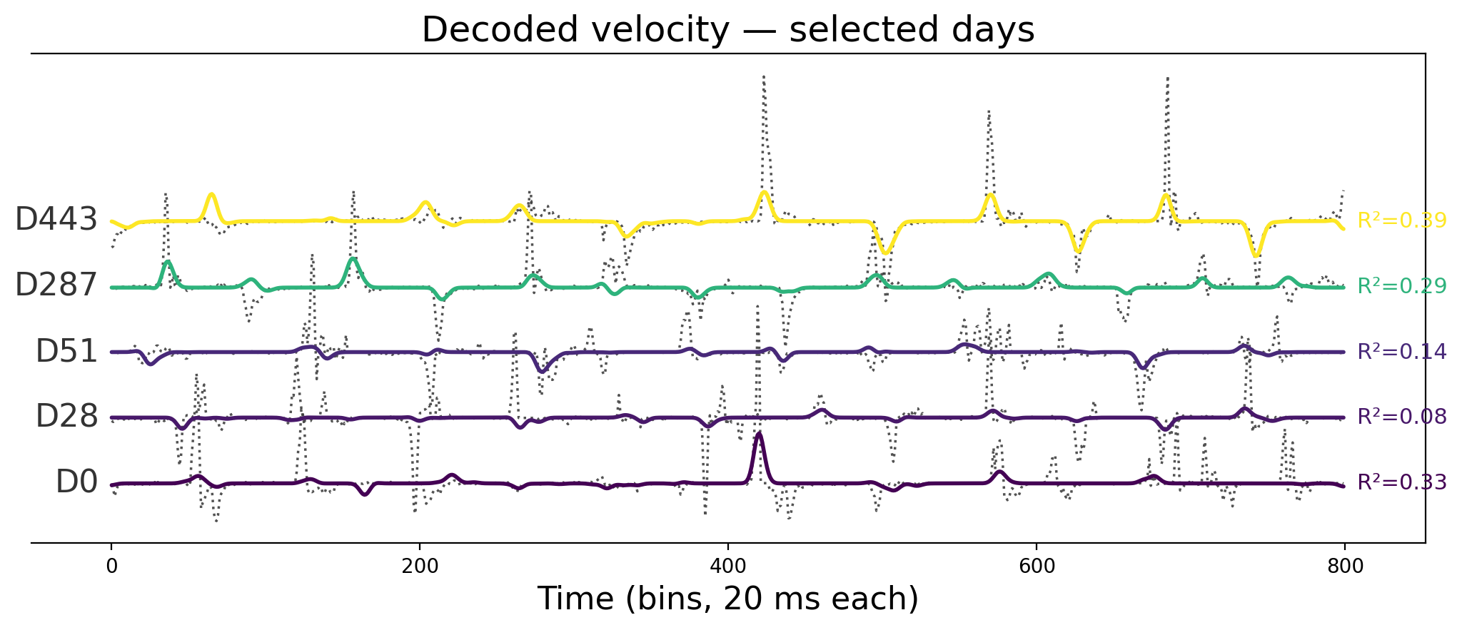
The R² values do not trend downward with implant age. The waterfall rows — including sessions recorded more than two years after others in the training pool — still show movement structure. This is the cross-session stability the linear baseline could not hold.
Performance Across All 30 Sessions
Per-session R² across the full dataset: minimum 0.158, maximum 0.435, mean 0.290 — see the timeline in the previous section.
No clear downward trend with implant age. Sessions near the end of the 3-year span perform comparably to early sessions. The variance across sessions (0.158–0.435) reflects differences in recording quality and task engagement, not a systematic drift of the kind that broke the static decoder in Part 1.
Limits
This result is real, but the scope is specific:
- Offline training. The MLP was trained on full sessions — it had access to all 30 sessions at training time. Deployment requires a decision about how many sessions to accumulate before training, and whether the model needs to be updated as the recording ages.
- TCR normalization not ablated. Part 2 ablated z-score vs. full r_norm for SBP. The contribution of TCR z_norm here isn't independently characterized — the horizon table compares the full joint model against SBP-only baselines, not SBP-alone MLP.
- NHP data. These results come from one non-human primate with a Utah array. Human implants, different array geometries, and different task structures may show different improvement profiles.
- No latency analysis beyond smoothing. The 60 ms causal smoother in the decoded traces approximates hardware constraints, but full real-time deployment latency depends on compute and pipeline overhead not characterized here.
The three parts, in one view
Wide table: on a narrow screen, scroll sideways to see all columns.
| Part | Question | Answer |
|---|---|---|
| Part 1 | Is raw SBP stationary across chronic sessions? | No. Monotonic drift, negative decoder transfer at every gap. |
| Part 2 | Does per-session normalization fix the representation? | Yes. r_norm shifts mean off-diagonal R² from −0.021 to +0.151. |
| Part 3 | Does a nonlinear cross-session decoder go further? | Yes. MLP on SBP + TCR maintains R² > 0.34 at every horizon including 1 month+. |
Part 1 through Part 3 trace the same arc on this dataset: raw drift and decoder failure, a within-session normalization that repairs the representation, and a jointly trained nonlinear decoder that holds performance across session pairs in the span analyzed here—under the assumptions and limits spelled out in each part.
References
- Magland, J. F., Ly, R., Rübel, O., & Dichter, B. K. (2025). Facilitating analysis of open neurophysiology data on the DANDI Archive using large language model tools. Scientific Data, 12, 285. https://doi.org/10.1038/s41597-025-06285-x
- Rübel, O., Tritt, A., Ly, R., Dichter, B. K., Ghosh, S., Niu, L., Baker, P., Soltesz, I., Ng, L., Svoboda, K., Frank, L., & Bouchard, K. E. (2022). The Neurodata Without Borders ecosystem for neurophysiological data science. eLife, 11, e78362. https://doi.org/10.7554/eLife.78362
The repository includes the analysis notebooks, the neurosignal package and related code, and HTML exports of those notebooks.
Code: github.com/radhakrishnanrishaban/ephys-signal-atlas · neurosignal v0.1.0